The Haskell School Of Expression

Polymorphic and Higher-Order Functions

In this chapter l will introduce two new important ideas. The first is polymorphism, the ability to consider entire families of types as one. Polymorphic data types are one source of this concept, which is then inherited by functions defined over these data types. The already familiar list is the most common example of a polymorphic data type, and it will be discussed at length in this chapter.

The second concept is the higher-order function, which is a function that can take one or more functions as arguments or return a function as a result (functions can also be placed in data structures, making the data constructors higher-order too). Together, polymorphic and higher-order functions substantially increase our expressive power and our ability to reuse code. You will see that both of these new ideas naturally follow the foundations that we have already built. (A more detailed discussion of polymorphic functions that operate on lists can be found in

Chapter 23.)

5.1 Polymorphic Types

In previous chapters we have seen examples of lists of many different kinds of elements - integers, floating-point numbers, points, characters, and even IO actions. You can well imagine situations requiring lists of other element types as well. Sometimes, however, we don't wish to be so particular about the precise type of the elements. For example, sup-pose we want to define a function length, which determines the number of elements in a list. We don't really care whether the list contains integers, characters, or even other lists. We imagine computing the length in exactly the same way in each case. The obvious definition is:

length [ ] =0

length (x : xs) = 1+ length xs

56

5.1 Polymorphic Types 57 ■

This definition is self-explanatory. We can read the equations as saying: “The lengthof the empty list is 0, and the lengthof a list whose first element is xand remainder is xs,is 1 plus the lengthof xs.”

But what should the type of lengthbe? Intuitively, what we'd like to say is that, for anytype a,the type of lengthis [a]→Integer.In Haskell we write this simply as:

length::[a]→Integer

DETAILS

Generic names for types, such as aabove, are called typevariables,and are uncapitalized to distinguish them from specific types such as Integer.

So lengthcan be applied to a list containing elements of anytype. For example:

length[l, 2, 3] ===> 3

length['a','b','c'] ===> 3

length“def” ===> 3

length[[1],[],[2,3,4]] ===> 3

Note that the type of the argument to lengthin the last example is [[Integer]];that is, a list of lists of integers.

Here are two other examples of polymorphic list functions, whichhappen to be predefined in Haskell:

head ::[a]→a

head(x:_)=x

tail ::[a]→[a]

tail(_:xs)=xs

As discussed briefly in Chapter I, these two functions take the ``head'' and ``tail,'' respectively, of any nonempty list:

head[I,2, 3] ===> I head['a','b','c']===>'a'tail[I,2, 3] ===> [2,3]tail['a','b','c']===>['b','c']

Functions suchas length,head,and tailare said to be polymorphic(polymeans manyand morphicrefers to the structure, or form,of objects). Polymorphic functions arise naturally when defining functions

58 Polymorphic and Higher-Order Functions

on lists and other structured data types. In the remainder of this chapter we will continue studying polymorphic lists, however, in Chapter 7, for example, we will look at another polymorphic data structure, namely a tree.

5.2 Abstraction Over Recursive Definitions

Recall from Section 4.l, the definition:

transList :: [Vertex] → [Point]

transList [ ] = [ ]

transList (p : ps) = trans p : transList ps

and from Section 3.1 the definition:

putCharList :: String → [IO ()]

putCharList [ ] = [ ]

putCharList (c : cs) = putChar c : putCharList cs

These two functions arose out of completely different contexts: the former in translating between graphics coordinate systems, and the latter in performing text IO. Yet surely these two definitions share something in common; surely there is a repeating pattern of operations here. But it is not quite like any of the examples that we studied in Section 1.4, and therefore, it is unclear how to apply the abstraction principle. What distinguishes this situation is a repeating pattern of recursion.

In discerning the nature of a repeating pattern, it's sometimes helpful to identify those things that aren't repeating (i.e., those things that are changing) because these will be the sources of parameterization: those values that must be passed as arguments to the abstracted function. In the case above, these changing values are the functions trans and putChar; let's consider them instances of a new name, f.If we then simply rewrite either of the above functions as a new function - let's call it (map f)- which takes an extra argument f,we arrive at:

map f [ ] = [ ]

map f (x : xs) = fx: map f xs

With this definition of map, we can now redefine transList and putCharList as:

transList :: [Vertex] → [Point]

transList ps = map trans ps

putCharList :: String → [IO ()] putCharList cs = map putChar cs

5.2 Abstraction Over Recursive Definitions 59

Note that these definitions are nonrecursive; the common pattern of recursion has been abstracted away and isolated in the definition of map. They are also very succinct; so much so, that it is often unnecessary to create new names for these functions at all. For example, in Section 3.1 we used putCharList to define putStr, whose complete definition was thus:

putStr :: String → IO ()

putStr s = sequence(putCharList s)

putCharList :: String → [IO ()]

putCharList [ ] = [ ]

putCharList (c : cs) = putChar c : putCharList cs

With map, however, we can define this much more directly and succinctly:

putStr :: String → IO ()

putStr s = sequence_ (map putChar s)

One of the powers of higher-order functions is that they permit concise yet easy-to-understand definitions such as this. You will see many similar examples throughout the remainder of the text.

To prove that the new versions of these two functions are equivalent to the old ones can be done via calculation, but requires a proof technique called induction, because of the recursive nature of the original function definitions. We will discuss inductive proofs in detail, including these two examples, in Chapter 11. In reality, induction is a formalization and generalization of the process above whereby we derived map from two of its instances.

5.2.1 Map is Polymorphic

What should the type of map be? Let's look first at its use in transList: it takes the function trans :: Vertex → Point as its first argument, a list of Vertexs as its second argument, and it returns a list of Points as its result. So its type must be:

map :: (Vertex → Point) → [Vertex] → [Point]

Yet a similar analysis of its use in putCharList reveals that map's type should be:

map :: (Char → IO ())→[Char]→[IO()]

This apparent anomaly can be resolved by noting that map, like length, head, and tail, does not really care what its list element types are, as long as its functional argument can be applied to them. Indeed,

60Polymorphic and Higher-Order Functions

map is polymorphic, and its most general type is: map :: (a→b)→[a]→[b]

This can be read: "map is a function that takes a function from any type a to any type b, and a list of a's, and returns a list of b's." The correspondence between the two a's and between the two b's is important: A function that converts Int's to Char's, for example, cannot be mapped over a list of Char's. It is easy to see that in the case of transList, a is instantiated as Vertex and b as Point, whereas in putCharList, a and b are instantiated as Char and IO (), respectively.

DETAlLS

It was mentioned in Chapter 1 that every expression in Haskell has an associated type. But with polymorphism, you might wonder if there is just one type for every expression. For example, map could have any of these types:

(a→b)→[a]→[b]

(Integer → b) → [Integer] → [b](a → Float) → [a] → [Float] (Char → Char) → [Char] → [Char]

and so on, depending on how it will be used. However, notice that the first of these types is in some fundamental sense more general than the other three. In fact, every expression in Haskell has a unique type known as its principal type: the least general type that captures all valid uses of the expression. The first type above is the principal type of map, because it captures all valid uses of map, yet is less general than, for example, the type a → b → c. As another example, the principal type of head is [a] → a; the types [b] → a, b → a, or even a are too general, whereas something like [Integer] → Integer is too specific.¹

5.2.2 Using map

Now that we can picture map as a polymorphic function, it is useful to look back on some of the examples we have worked through to see if

¹ The existence of unique principal types is the hallmark feature of the Hindley-Milner type system (Hindley, 1969; Milner, 1978), which forms the basis of the type systems of Haskell, ML (Milner et al., 1990), and many other functional languages

(Hudak, 1989).

5.2 AbstractionOverRecursiveDefinitions 61 ■

there are any situations where map might have been helpful. For starters, recall from Section 1.4.3 the definition of totalArea:

totaiArea = listSum [circleArea r1, circleArea r2, circleArea r3]

lt should be clear that this can be rewritten as:

totaiArea = listSum (map circleArea [r1, r2, r3])

A simple calculation is all that is needed to show that these are the same:

map circleArea [r1, r2, r3] ==> circleArea r1 : map circleArea [r2, r3] ==> circleArea r1 : circleArea r2 : map circleArea [r3] ==> circleArea r1 : circleArea r2 : circleArea r3 : map circleArea [ ] ==> circleArea r1 : circleArea r2 : circleArea r3 : [ ] ==> [circleArea r1, circleArea r2, circleArea r3]

Also recall from Section 4.3 the following function for drawing a list of colored shapes:

type ColoredShapes = [(Color, Shape)]

drawShapes :: Window → ColoredShapes → IO () drawShapes w [ ]

= return () drawShapes w ((c,s) : cs)

= do draw w (withColor c (shapeToGraphic s))drawShapes w cs

Using the sequence_ function introduced in Section 3.1, this can be rede-fined as:

drawShapes w css

= sequence_ (map aux css)

where aux (c,s)= draw w (withColor c (shapeToGraphic s))

This example demonstrates that map can be used effectively for IO tasks. I would argue that this definition is clearer than the earlier one, because it abstracts away nicely the repeated IO operation in the function aux. A suitable reading of the above code might be: "Sequence together the successive actions of aux on each of the colored shapes." That reading is less obvious from the earlier recursive definition.

62Polymorphic and Higher-Order Functions

As a final example of the use of map, let's generate a list of eight concentric circles:

conCircles = map circle [2.4, 2.1..0.3]

DETAlLS

A list [a, b..c] is called an arithmetic sequence, and is special syntax for the list [a,a+d,a+ 2 * d,...,cl where d=b-a.Thus, [2.4, 2.1..0.3] is shorthand for the list [2.4, 2.1, 1.8, 1.5, 1.2, 0.9, 0.6, 0.3].

We can pair each of these circles with a color:

coloredCircles = zip [Black, Blue, Green, Cyan, Red, Magenta, Yellow, White] conCircles

DETAlLS

The PreludeList function zip (see Chapter 23) takes two lists and returns a list of the pairwise elements. For example:

zip [1,2, 3] [4, 5, 6] ==> [(1,4), (2, 5), (3,6)]

It is defined as:

zip :: (a→b→c)→[a]→[b]→ [c]

zip (a : as) (b : bs) = (a,b) : zip as bs

zip__ =[]

(Recall that _ is a wildcard pattern, which matches any argument.)

This list of color/circle pairs can then be drawn using drawShapes:

main

= runGraphics (

do w ← openWindow “Bull's Eye”(xWin, yWin) drawShapes w coloredCircles spaceClose w

)

Note that coloredCircles is ordered largest circle first; thus draw-Shapes draws them in order of decreasing size (otherwise the larger circles would obscure the smaller ones!). A snapshot of main is shown in

Fig. 5.1.

5.3 Append ■ 63■

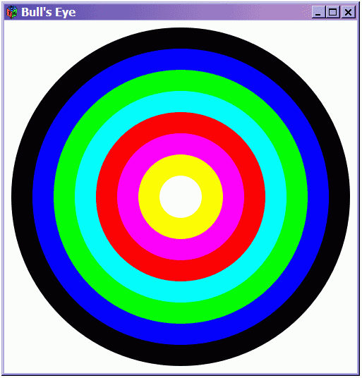
Figure 5.1 : A Bull's Eye

In the remainder of the text we will be looking for opportunities to use map directly rather than after-the-fact. indeed, there will be many such opportunities.

5.3 Append

Let's now consider the problem of concatenating or appending two lists together; that is, creating a third list that consists of all the elements from the first list followed by all of the elements of the second. Once again the type of list elements does not matter, so we will define this as

polymorphic infix operator ( ++ ) :

(++) :: [a]→[a]→[a]

For example, here are two uses of (++) on different types:

[1, 2, 3] ++[4, 5, 6] ===> [1,2,3,4,5,6] "hello" ++ "world" ===> "hello world"

■ 64■ Polymorphic and Higher-Order Functions

As usual, we can approach this problem by considering the various possibilities that could arise as input. But in the case of (++) we are given two inputs - so which do we consider first? In general, this is not an easy question, but in the case of (++) we can get a hint about what to do by noting that the result contains firstly all of the elements from the first list. So let's consider the first list first: It could be empty, or nonempty. If it is empty the answer is easy:

[]++ys= ys

and if it is not empty the answer is also straightforward:

(x:xs)++ys=x:(xs++ys)Note the recursive use of (++). Our full definition is thus:

(++) :: [a]→[a]→[a]

[]++ys=ys (x:xs)++ys=x:(xs++ys)

If we were to have considered instead the second list first, the first equation would still be easy:

xs++ [ ] = xs but the second is not so obvious:

xs ++ (y:ys)= ?? So you see, we made the right choice to begin with.

5.3.1 The Efficiency and Fixity of Append

In Chapter 11 we will prove the following simple property about (++):

(xs++ys)++zs = xs ++(ys++zs)

That is, (++) is associative.

But what about the efficiency of the left-hand and right-hand sides of this equation? It is easy to see via calculation that appending two lists together takes a number of steps proportional to the length of the first

5.4 Fold 65

list (indeed the second list is not evaluated at all). For example:

[1, 2, 3] ++ xs ==> 1:([2,3]++xs) ==> 1:2:([3]++xs) ==> 1:2:3: ([] ++xs) ==> 1 : 2 : 3 : xs

Therefore, the evaluation of xs ++ (ys ++ zs) takes a number of steps proportional to the length of xs plus the length of ys. But what about (xs ++ ys) ++ zs? The leftmost append will take a number of steps proportional to the length of xs, but then the rightmost append will require a number of steps proportional to the length of xs plus the length of ys, for a total cost of:

2 * length xs + length ys

Thus, xs ++ (ys ++ zs) is more efficient than (xs ++ ys) ++ zs. This is why the Standard Prelude defines the fixity of (++) as:

infixr5 ++

In other words, if you just write xs ++ ys ++ zs, you will get the most efficient association, namely the right association xs ++ (ys ++ zs). In the next section a more dramatic example of this property will be demonstrated.

5.4 Fold

As another example of applying the abstraction principle to a pair of recursive definitions (such as we did for map), recall the definition of listSum in Section 1.4.3:

listSum :: [Float] → Float

listSum [ ] =0

listSum (x : xs) = x + listSum xs

Now let's suppose that we need to compute the product of the elements of a list. For example, suppose the list contains the number of different colors, sizes, shapes, and so on of boxes that are sold by some company, and we wish to compute exactly the total number of unique boxes. This is simply the product of the numbers in the list. And so we

66Polymorphic and Higher-Order Functions

write:

listProd :: [Float] → Float

listProd [ ] =1

listProd (x : xs) = x * listProd xs

Surely, these two definitions share something in common, as did transList and putCharList. Using the process that we used to discover map, let's first identify those things that are changing. There are two pairs: the 0 and 1 values (for which we'll use the generic name init, for ``initial value”), and the (+) and (*) operators (for which we'll use the generic name op, for ``operator''). If we now rewrite either of the above functions as a new function - let's call it fold - that takes extra arguments op and init, we arrive at:²

fold op init [ ] = init

fold op init (x : xs) = x `op` fold op init xs

DETAILS

I chose infix application for op to reflect better the structure of the repeating pattern that we are abstracting.

From this it appears that fold's type should be:

fold :: (Float → Float → Float) → Float → [Float] → Float

With this definition of fold we can now rewrite the definitions of listSum and listProd as:

listSum, listProd :: [Float] → Float listSum xs = fold (+) 0 xs

listProd xs = fold ( * ) 1 xs

DETAILS

Just as we can turn a function into an operator by enclosing it in backquotes, we can turn an operator into a function by enclosing it in parentheses. This is required in order to pass an operator as a value to another function, as

² The use of the name “fold”for this function is historical, and has little to do with the use of “fold” and “unfold” to describe steps in a calculation.

5.4 Fold ■ 67

in the examples above. (If we wrote fold +0 xs instead of fold (+)0 xs it would look like we were trying to add fold to 0 xs, which is nonsensical and ill-typed.)

In Chapter 11 we will use induction to prove that these new definitions are equivalent to the old ones.

The function fold, like map, is a highly useful, and reusable, function, as you will see through many examples in this text. Indeed, it too is polymorphic, for note that it does not depend on the type of the list elements. Its most general type - somewhat trickier than that for map -is:

fold :: (a→b→b)→b→[a]→b

This allows us to use fold whenever we need to ``collapse'' a list of elements using a binary (i.e., two-argument) operator.

5.4.1 Haskell's Folds

Haskell actually defines two versions of fold in the Standard Prelude. The first is called foldr (``fold-from-the-right''), which is defined the same as our fold:

foldr :: (a→b→b)→b→[a]→b

foldr op init [ ] = init

foldr op init (x : xs) = x `op` foldr op init xs

A good way to think about foldr is that it replaces all occurrences of the list operator (:) with its first argument (a function), and replaces [ ] with its second argument. In other words:

foldr op init (x1 : x2 : . . . : xn : [ ]) ===> x1 `op` (x2 `op` (...(xn `op` init) . . .))

This might help you to understand the type of foldr better, and also explains its name: the list is ``folded from the right.'' Stated another way, for any list xs, the following always holds:³

foldr (:) [ ] xs ===> xs

³ We will formally prove this in Chapter 11.

68Polymorphic and Higher-Order Functions

Haskell's second version of fold is called foldl:

foldl :: (b→a→b)→b→[a]→b

foldl op init [ ] = init

foldl op init (x : xs) = foldl op (init `op` x) xs

A good way to think about foldl is to imagine ``folding the list from the

left'':

foldl op init (x1 : x2 : . . . : xn : [ ])===>(. . . ((init `op` x1) `op` x2) . . .) `op` xn

5.4.2 Why Two Folds?

Note that if we had used foldl instead of foldr in the definitions given earlier for listSum and listProd:

listSum, listProd :: [Integer] → Integer listSum xs = foldl (+) 0 xs

listProd xs = foldl ( * ) 1 xs

then nothing would have changed; foldr and foldl give the same result. Indeed, judging from their types, it looks like the only difference between foldr and foldl is that each takes its arguments in a different order.

So why does Haskell define two versions of fold? It turns out that there are situations where using one is more efficient, and possibly ``more defined,'' than the other. (By more defined, I mean that the function terminates on more values of its input domain.)

Probably the simplest example of this is a generalization of the associativity of (++) discussed in the last section. Suppose that we wish to collapse a list of lists into one list. The Standard Prelude defines the polymorphic function concat for this purpose:

concat :: [[a]]→[a] concat xss = foldr (++)[] xss

For example:

concat [[1], [3,4], [], [5,6]] ==> [1, 2, 3,4, 5, 6]

More importantly, from the earlier discussion it should be clear that this property holds:

concat [xs1, xs2, . . . , xsn] ==> foldr (++) [ ] [xs1, xs2, . . . , xsn] ==> xs1 ++ (xs2 ++(... (xn++[]))...)

5.5 A Final Example: Reverse ■ 69■

The total cost of this computation is proportional to the sum of the lengths of all the lists. If each list has the same length len, then this cost is n * len.

On the other hand, if we had defined concat this way:

slowConcat xss = foldl (++) [] xss

then we have:

slowConcat [xs1, xs2, ..., xsn]

==> foldl (++) [] [xsl, xs2, ..., xsn]

==> (...(([] ++ xl) ++ x2) ...) ++ xn

If each list has the same length len, then the cost of this computation will be:

len + (len + len) + (len + len + len) +...+(n-1)*len==> n * (n- 1)* len

which is considerably worse than n * len. Thus, the choice of foldr in the definition of concat is quite important.

Similar examples can be given to demonstrate that foldl is sometimes more efficient than foldr. On the other hand, in many cases the choice does not matter at all (consider, for example, (+)). The moral of all this is that care must be taken in the choice between foldr and foldl if efficiency is a concern.

A Final Example: Reverse

As a final example, consider the problem of creating a list that is the reverse of a given list, which I will capture in a function called reverse. For example, reverse [1,2,3]is [3,2,l].Thus, reverse takes a single list argument, whose possibilities are the normal ones for a list: It is either empty, or it is not. And so we write:

reverse :: [a]→[a]

reverse []=[]

reverse (x:xs) = reverse xs ++[x]

This, in fact, is a perfectly good definition for reverse. It is certainly clear, except for one small problem: It is terribly inefficient! To see why, first note that the number of steps needed to compute xs ++ys is proportional to the length of xs. Now suppose that the list argument to

70 Polymorphic and Higher-Order Functions

reverse has length n. The recursive call to reverse will return a list of length n - 1, which is the first argument to (++). Thus, the cost to reverse a list of length of n will be proportional to n - 1 plus the cost to reverse a list of length n - 1. So the total cost is proportional to (n-1) + (n-2) + ... + 1 = n(n- 1)/2, which in turn is proportional to the square of n. Can we do better than this? Yes we can.

There is another algorithm for reversing a list, which goes something like this: Take the first element, and put it at the front of an empty auxiliary list; then take the next element and add it to the front of the auxiliary list (thus the auxiliary list now consists of the first two elements in the original list, but in reverse order); then do this again and again until you reach the end of the original list. At that point the auxiliary list will be the reverse of the original one.

This algorithm can be expressed recursively, but the auxiliary list implies that we need a function that takes two arguments - the original list and the auxiliary one - yet reverse only takes one. So we create an auxiliary function rev:

reverse xs = rev [ ] xs whererev acc [ ] = acc

rev acc (x : xs) = rev (x : acc) xs

The auxiliary list is the first argument to rev, and is called acc because it behaves as an ``accumulator'' of the intermediate results. Note how it is returned as the final result once the end of the original list is reached.

A little thought should convince you that this function does not have the quadratic (n²)behavior of the first algorithm, and indeed can be shown to execute a number of steps that is directly proportional to the length of the list, which we can hardly expect to improve upon.

But now, compare the definition of rev with the definition of foldl:

foldl op init [ ] = init

foldl op init (x : xs) = foldl op (init `op` x) xs

They are somewhat similar. In fact, suppose we were to slightly rewrite rev, yielding:

rev op acc [ ] = acc

rev op acc (x : xs) = rev op (acc `op` x) xs

Now rev looks exactly like foldl, and the question becomes whether or not there is a function that can be substituted for op that would make

5.6 Errors ■ 71 ■

the latter definition of rev equivalent to the former one. Indeed there is:

revOp a b = b : a For note that:

acc `revOp` x ==> revOp acc x ==> x : acc

So reverse can be rewritten as:

reverse xs = rev revOp [ ] xs whererev op acc [ ] = acc

rev op acc (x : xs) = rev op (acc `op` x) xs

which is the same as:

reverse xs = foldl revOp [ ] xs

5.6 Errors

Recall the Shape data type from Chapter 2. What if negative side lengths are used with the Rectangle constructor, or negative radii with the Ellipse? This may or may not make sense, depending on the application. In Chapter 8, I will argue that in some cases it does make sense, but careful consideration of these potentially anomalous situations is important. If negative side lengths are used, area may compute a negative area. And what will happen when such a figure is drawn?

There are many ways to deal with such situations, again depending on the application, but sometimes we wish to literally stop the program, signaling to the user that some kind of an error has occurred. In Haskell this is done with the Standard Prelude function error :: String → a. Note that error is polymorphic, meaning that it can be used with any data

type. The value of the expression error s is

, the completely undefined,

or “bottom” value. As an example of its use, suppose that we wish to signal an error when the area of a rectangle with negative side lengths is attempted. We can write:

area (Rectangle s1 s2)

|s1>=0∓mp;∓mp;s2>=0=s1*s2

| otherwise = error “area: negative side lengths”

The effect of this change is that if the anomalous situation arises, the program will terminate immediately, and the string “area: negative side lengths'' will be printed to the standard output area.

■72■Polymorphic and Higher-Order Functions

DETAILS

(∓mp;∓mp;) and (||) are Haskell's Boolean “and" and “or" operators, respectively. b1∓mp;∓mp; b2 should be read “b1and b2“; similarly for (||). They are defined

in the Standard Prelude as:

(∓mp;∓mp;),(||)::Bool→Bool→BoolTrue∓mp;∓mp;x=xFalse∓mp;∓mp;_=FalseTrue||_=TrueFalse||x=x

Just as we used the constructors in the Shapedata type for pattern matching in previous chapters, here we are pattern matching against the constructors Trueand Falseof the Booldata type.

Exercise 5.1 Rewrite the equation for the area of a polygon given in Section 2.2 in a higher-order, nonrecursive way, using operators such as map, fold, and so on.

Exercise 5.2 What is the principal type of each of the following expressions:

map map

foldl foldl

map foldl

Exercise 5.3 Rewrite the definition of length nonrecursively.

Exercise 5.4 Using higher-order functions that we have now defined, fill in the two missing functions, f1 and f2, in the evaluation below so that it is valid:

f1(f2(*)[1,2,3,4])5 ==> [5,10,15,20]

Exercise 5.5 Define a function that behaves as each of the following:

1. Doubles each number in a list. For example:

doubleEach [1, 2, 3] ===> [2, 4, 6]

2. Pairs each element in a list with that number and one plus that number. For example:

pairAndOne [1, 2, 3] ===> [(1, 2), (2, 3), (3, 4)]

5.6 Errors 73

3. Adds together each pair of numbers in a list. For example:

addEachPair [(1, 2), (3, 4), (5, 6)] ===> [3,7,11]

In this exercise and the two that follow, give both recursive and (if possible) nonrecursive definitions, and be sure to include type signatures.

Exercise 5.6Define a function maxList that computes the maximum element of a list. Define minList analogously.

Exercise 5.7Define a function that adds “pointwise” the elements of a list of pairs. For example:

addPairsPointwise [(1, 2), (3, 4), (5, 6)] ===> (9, 12)

Exercise 5.8Freddie the Frog wants to communicate privately with his girlfriend Francine by encrypting messages sent to her. Frog brains are not large, so they agree on this simple strategy: Each character in the text shall be converted to the character ``one greater'' than it, based on the representation described below (with wrap-around from 255 to 0). Define functions encrypt and decrypt that will allow Freddie and Francine to communicate using this strategy.

Hint: Characters are often represented inside a computer as some kind of an integer; in the case of Haskell, a 16-bit unicode representation is used. For this exercise, you will want to use two Haskell functions, toEnum and fromEnum. The first will convert an integer into a character, the second will convert a character into an integer.

Exercise 5.9Suppose you are given a nonnegative integer amt representing a sum of money, and a list of coin denominations [v1, v2, ..., vn],each being a positive integer. Your job is to make change for amt using the coins in the coin supply. Define a function makeChange to solve this problem. For example, your function may behave like this:

makeChange 99 [5, 1] ==> [19, 4]

where 99 is the amount and [5, 1] represents the types of coins (say, nickels and pennies in U.S. currency) that we have. The answer [19, 4] means that we can make the exact change with 19 five-unit coins and 4 single-unit coins; this is the best (in terms of the total number of coins) possible solution.

To make things slightly easier, you may assume that the list representing the coin denominations is given in descending order, and that the single-unit coin is always one of the coin types.